深度学习归一化方法[一] Batch Normalization

论文: https://arxiv.org/pdf/1502.03167.pdf

Batch Normalization

对模型的初始输入进行归一化处理，可以提高模型训练收敛的速度;对神经网络内层的数据进行归一化处理，同样也可以达到加速训练的效果。Batch Normalization 就是归一化的一个重要方法。以下将介绍BN是如何归一化数据，能起到什么样的效果以及产生该效果的原因展开介绍。

1. Batch Normalization原理

(一)前向传播

在训练阶段：
(1)对于输入的mini-batch数据 $B=\left\{x_{1\dots m}\right\}$B={x1…m​}，假设shape为(m, C, H, W),计算其在Channel维度上的均值和方差：
$\begin{array}{cc}{\displaystyle {\mu }_B}& {\displaystyle =\frac{1}{m}\sum _{i=1}^m{x}_i}\\ {\displaystyle {\sigma }_B^2}& {\displaystyle =\frac{1}{m}\sum _{i=1}^m{(x_i-{\mu }_B)}^2}\end{array}$μB​σB2​​=m1​i=1∑m​xi​=m1​i=1∑m​(xi​−μB​)2​
(2)根据计算出来的均值和方差，归一化mini-Batch中每一个样本：
${\widehat{x}}_i=\frac{x_i-{\mu }_B}{\sqrt{{\sigma }_B^2+ϵ}}$x i​=σB2​+ϵ ​xi​−μB​​
(3)最后，对归一化后的数据进行一次平移+缩放变换：
$y_i=\gamma {\widehat{x}}_i+\beta \equiv B{N}_{\gamma ,\beta }\left(x_i\right)$yi​=γx i​+β≡BNγ,β​(xi​)
$\gamma 、\beta$γ、β是需要学习的参数。

在测试阶段：
使用训练集中数据的 ${\mu }_B$μB​和 ${\sigma }_B^2$σB2​无偏估计作为测试数据归一化变换的均值和方差：
$\begin{array}{c}E\left(x\right)=E_B\left({\mu }_B\right)\\ \mathrm{Var}\left(x\right)=\frac{m}{m-1}{E}_B\left({\sigma }_B^2\right)\end{array}$E(x)=EB​(μB​)Var(x)=m−1m​EB​(σB2​)​
通过记录训练时每一个mini-batch的均值和方差最后取均值得到。
而在实际运用中，常动态均值和动态方差，通过一个动量参数维护:
$\begin{array}{cc}{\displaystyle r{\mu }_{B_t}}& {\displaystyle =\beta r{\mu }_{B_{t-1}}+(1-\beta ){\mu }_B}\\ {\displaystyle r{\sigma }_{B_t}^2}& {\displaystyle =\beta r{\sigma }_{B_{t-1}}^2+(1-\beta ){\sigma }_B^2}\end{array}$rμBt​​rσBt​2​​=βrμBt−1​​+(1−β)μB​=βrσBt−1​2​+(1−β)σB2​​
$\beta$β一般取0.9.
因此可以得到测试阶段的变换为：
$y=\gamma \frac{x-E\left(x\right)}{\sqrt{Var\left(x\right)+ϵ}}+\beta$y=γVar(x)+ϵ ​x−E(x)​+β
或：
$y=\gamma \frac{x-r{\mu }_{B_t}}{\sqrt{r{\sigma }_{B_{t-1}}^2+ϵ}}+\beta$y=γrσBt−1​2​+ϵ ​x−rμBt​​​+β

（二）反向传播（梯度计算）
计算梯度最好的方法是根据前向传播的推导公式，构造出计算图，直观反映变量间的依赖关系。
前向传播公式：
$\begin{array}{cc}{\displaystyle {\mu }_B}& {\displaystyle =\frac{1}{m}\sum _{i=1}^m{x}_i}\\ {\displaystyle {\sigma }_B^2}& {\displaystyle =\frac{1}{m}\sum _{i=1}^m{(x_i-{\mu }_B)}^2}\\ {\displaystyle {\widehat{x}}_i}& {\displaystyle =\frac{x_i-{\mu }_B}{\sqrt{{\sigma }_B^2+ϵ}}}\\ {\displaystyle y_i}& {\displaystyle =\gamma {\widehat{x}}_i+\beta }\end{array}$μB​σB2​x i​yi​​=m1​i=1∑m​xi​=m1​i=1∑m​(xi​−μB​)2=σB2​+ϵ ​xi​−μB​​=γx i​+β​
计算图：

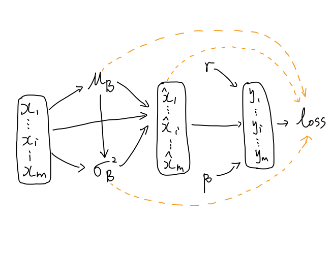
黑色线表示前向传播的关系，橙色线表示反向传播的关系
利用计算图计算梯度的套路：

• 先计算离已知梯度近的变量的梯度，这样在计算远一点变量的梯度时，可能可以直接利用已经计算好的梯度；
• 一个变量有几个出边（向外延伸的边），其梯度就由几项相加。

当前已知 $\frac{\partial l}{\partial y_i}$∂yi​∂l​,要计算loss对图中每一个变量的梯度.
按照由近及远的方法,依次算 $\gamma ,\beta ,\widehat{x_i}$γ,β,xi​^​.由于 ${\sigma }_B^2$σB2​依赖于 ${\mu }_B$μB​,所以先计算 ${\sigma }_B^2$σB2​,再计算 ${\mu }_B$μB​,最后计算$x_i
$
$\gamma$γ:表面一个出边,实际上有m个出边,因为每一个 $y_i$yi​的计算都与 $\gamma$γ有关,因此
$\begin{array}{cc}{\displaystyle \frac{\partial l}{\partial \gamma }}& {\displaystyle =\sum _{i=1}^m\frac{\partial l}{\partial y_i}\frac{\partial y_i}{\partial \gamma }}\\ {\displaystyle }& {\displaystyle =\sum _{i=1}^m\frac{\partial l}{\partial y_i}\widehat{x_i}}\end{array}$∂γ∂l​​=i=1∑m​∂yi​∂l​∂γ∂yi​​=i=1∑m​∂yi​∂l​xi​^​​
$\beta$β:同理
$\begin{array}{cc}{\displaystyle \frac{\partial l}{\partial \beta }}& {\displaystyle =\sum _{i=1}^m\frac{\partial l}{\partial y_i}\frac{\partial y_i}{\partial \beta }}\\ {\displaystyle }& {\displaystyle =\sum _{i=1}^m\frac{\partial l}{\partial y_i}}\end{array}$∂β∂l​​=i=1∑m​∂yi​∂l​∂β∂yi​​=i=1∑m​∂yi​∂l​​
$\widehat{x_i}$xi​^​:一条出边
$\begin{array}{cc}{\displaystyle \frac{\partial l}{\partial \widehat{x_i}}}& {\displaystyle =\frac{\partial l}{\partial y_i}\frac{\partial y_i}{\partial \widehat{x_i}}}\\ {\displaystyle }& {\displaystyle =\frac{\partial l}{\partial y_i}\gamma }\end{array}$∂xi​^​∂l​​=∂yi​∂l​∂xi​^​∂yi​​=∂yi​∂l​γ​
${\sigma }_B^2$σB2​:m条出边,每一个 $\widehat{x_i}$xi​^​的计算都依赖于 ${\sigma }_B^2$σB2​.找到其到loss的路径: ${\sigma }_B^2\to \widehat{x_i}\to y_i\to loss$σB2​→xi​^​→yi​→loss,由于 $\widehat{x_i}$xi​^​关于loss的梯度已经计算好了,所以路径为 ${\sigma }_B^2\to \widehat{x_i}\to loss$σB2​→xi​^​→loss,因此
$\begin{array}{cc}{\displaystyle \frac{\partial l}{\partial {\sigma }_B^2}}& {\displaystyle =\sum _{i=1}^m\frac{\partial l}{\partial \widehat{x_i}}\frac{\widehat{x_i}}{{\sigma }_B^2}}\\ {\displaystyle }& {\displaystyle =\sum _{i=1}^m\frac{\partial l}{\partial \widehat{x_i}}\frac{-1}{2}(x_i-{\mu }_B)({\sigma }_B^2+ϵ{)}^{-\frac{3}{2}}}\end{array}$∂σB2​∂l​​=i=1∑m​∂xi​^​∂l​σB2​xi​^​​=i=1∑m​∂xi​^​∂l​2−1​(xi​−μB​)(σB2​+ϵ)−23​​
${\mu }_B$μB​出边有m + 1条.路径: ${\mu }_B\to {\sigma }_B^2\to loss$μB​→σB2​→loss, ${\mu }_B\to \widehat{x_i}\to loss$μB​→xi​^​→loss,因此;
$\begin{array}{cc}{\displaystyle \frac{\partial l}{\partial {\mu }_B}}& {\displaystyle =\frac{\partial l}{\partial {\sigma }_B^2}\frac{{\sigma }_B^2}{\partial {\mu }_B}+\sum _{i=1}^m\frac{\partial l}{\partial \widehat{x_i}}\frac{\partial \widehat{x_i}}{\partial {\mu }_B}}\\ {\displaystyle }& {\displaystyle =\frac{\partial l}{\partial {\sigma }_B^2}\frac{-2}{m}\sum _{i=1}^m(x_i-{\mu }_B)+\sum _{i=1}^m\frac{\partial l}{\partial \widehat{x_i}}\left(\frac{-1}{\sqrt{{\sigma }_B^2+ϵ}}\right)}\end{array}$∂μB​∂l​​=∂σB2​∂l​∂μB​σB2​​+i=1∑m​∂xi​^​∂l​∂μB​∂xi​^​​=∂σB2​∂l​m−2​i=1∑m​(xi​−μB​)+i=1∑m​∂xi​^​∂l​(σB2​+ϵ ​−1​)​
$x_i$xi​:有3条边,路径: $x_i\to {\mu }_B\to loss$xi​→μB​→loss, $x_i\to {\sigma }_B^2\to loss$xi​→σB2​→loss, $x_i\to \widehat{x_i}\to loss$xi​→xi​^​→loss
$\begin{array}{cc}{\displaystyle \frac{\partial l}{\partial x_i}}& {\displaystyle =\frac{\partial l}{\partial {\mu }_B}\frac{\partial {\mu }_B}{\partial x_i}+\frac{\partial l}{{\sigma }_B^2}\frac{{\sigma }_B^2}{\partial x_i}+\frac{\partial l}{{\widehat{x}}_i}\frac{{\widehat{x}}_i}{\partial x_i}}\\ {\displaystyle }& {\displaystyle =\frac{\partial l}{\partial {\mu }_B}\frac{1}{m}+\frac{\partial l}{\partial {\sigma }_B^2}\frac{-2}{m}(x_i-{\mu }_B)+\frac{\partial l}{\partial {\widehat{x}}_i}\frac{1}{\sqrt{{\sigma }_B^2+ϵ}}}\end{array}$∂xi​∂l​​=∂μB​∂l​∂xi​∂μB​​+σB2​∂l​∂xi​σB2​​+x^i​∂l​∂xi​x^i​​=∂μB​∂l​m1​+∂σB2​∂l​m−2​(xi​−μB​)+∂x^i​∂l​σB2​+ϵ ​1​​

求导完毕!!!
附上代码实现:

def batchnorm_forward(x, gamma, beta, bn_param):
    """ Forward pass for batch normalization. Input: - x: Data of shape (N, D) - gamma: Scale parameter of shape (D,) - beta: Shift paremeter of shape (D,) - bn_param: Dictionary with the following keys: - mode: 'train' or 'test'; required - eps: Constant for numeric stability - momentum: Constant for running mean / variance. - running_mean: Array of shape (D,) giving running mean of features - running_var Array of shape (D,) giving running variance of features Returns a tuple of: - out: of shape (N, D) - cache: A tuple of values needed in the backward pass """
    mode = bn_param['mode']
    eps = bn_param.get('eps', 1e-5)
    momentum = bn_param.get('momentum', 0.9)

    N, D = x.shape
    running_mean = bn_param.get('running_mean', np.zeros(D, dtype=x.dtype))
    running_var = bn_param.get('running_var', np.zeros(D, dtype=x.dtype))

    out, cache = None, None
    
    if mode == 'train':

        sample_mean = np.mean(x, axis=0)
        sample_var = np.var(x, axis=0)
        out_ = (x - sample_mean) / np.sqrt(sample_var + eps)

        running_mean = momentum * running_mean + (1 - momentum) * sample_mean
        running_var = momentum * running_var + (1 - momentum) * sample_var

        out = gamma * out_ + beta
        cache = (out_, x, sample_var, sample_mean, eps, gamma, beta)

    elif mode == 'test':

        scale = gamma / np.sqrt(running_var + eps)
        out = x * scale + (beta - running_mean * scale)

    else:
        raise ValueError('Invalid forward batchnorm mode "%s"' % mode)

    # Store the updated running means back into bn_param
    bn_param['running_mean'] = running_mean
    bn_param['running_var'] = running_var

    return out, cache

def batchnorm_backward(dout, cache):
    """ Backward pass for batch normalization. Inputs: - dout: Upstream derivatives, of shape (N, D) - cache: Variable of intermediates from batchnorm_forward. Returns a tuple of: - dx: Gradient with respect to inputs x, of shape (N, D) - dgamma: Gradient with respect to scale parameter gamma, of shape (D,) - dbeta: Gradient with respect to shift parameter beta, of shape (D,) """
    dx, dgamma, dbeta = None, None, None

    out_, x, sample_var, sample_mean, eps, gamma, beta = cache

    N = x.shape[0]
    dout_ = gamma * dout
    dvar = np.sum(dout_ * (x - sample_mean) * -0.5 * (sample_var + eps) ** -1.5, axis=0)
    dx_ = 1 / np.sqrt(sample_var + eps)
    dvar_ = 2 * (x - sample_mean) / N

    # intermediate for convenient calculation
    di = dout_ * dx_ + dvar * dvar_
    dmean = -1 * np.sum(di, axis=0)
    dmean_ = np.ones_like(x) / N

    dx = di + dmean * dmean_
    dgamma = np.sum(dout * out_, axis=0)
    dbeta = np.sum(dout, axis=0)

    return dx, dgamma, dbeta

2. Batch Normalization的效果及其证明

(一) 减小Internal Covariate Shift的影响, 权重的更新更加稳健.
对于不带BN的网络,当权重发生更新后,神经元的输出会发生变化,也即下一层神经元的输入发生了变化.随着网络的加深,该影响越来越大,导致在每一轮迭代训练时,神经元接受的输入有很大的变化,此称为Internal Covariate Shift. 而BatchNormalization通过归一化和仿射变换(平移+缩放),使得每一层神经元的输入有近似的分布.
假设某一层神经网络为:
$H_{i+1}=W{H}_i+b$Hi+1​=WHi​+b
对权重的导数为:
$\frac{\partial l}{\partial W}=\frac{\partial l}{\partial H_{i+1}}{H_i}^T$∂W∂l​=∂Hi+1​∂l​Hi​T
对权重进行更新:
$W\leftarrow W-\eta \frac{\partial l}{\partial H_{i+1}}{H_i}^T$W←W−η∂Hi+1​∂l​Hi​T
可见,当上一层神经元的输入( $H_i$Hi​)变化较大时,权重的更新变化波动大.
(二)batch Normalization具有权重伸缩不变性,可以有效提高反向传播的效率,同时还具有参数正则化的效果.
记BN为:
$Norm\left(Wx\right)==g\cdot \frac{Wx-\mu }{\sigma }+b$Norm(Wx)==g⋅σWx−μ​+b
为什么具有权重不变性? $\downarrow$↓
假设权重按照常量 $\lambda$λ进行伸缩,则其对应的均值和方差也会按比例伸缩,于是有:
$\begin{array}{cc}{\displaystyle Norm\left(W^{\prime }x\right)}& {\displaystyle =g\cdot \frac{W^{\prime }x-{\mu }^{\prime }}{{\sigma }^{\prime }}+b}\\ {\displaystyle }& {\displaystyle =g\cdot \frac{\lambda Wx-\lambda \mu }{\lambda \sigma }+b}\\ {\displaystyle }& {\displaystyle =g\cdot \frac{Wx-\mu }{\sigma }+b}\\ {\displaystyle }& {\displaystyle =Norm\left(Wx\right)}\end{array}$Norm(W′x)​=g⋅σ′W′x−μ′​+b=g⋅λσλWx−λμ​+b=g⋅σWx−μ​+b=Norm(Wx)​

为什么能提高反向传播的效率? $\downarrow$↓
考虑权重发生伸缩后,梯度的变化:
为方便(公式打累了),记 $y=Norm\left(Wx\right)$y=Norm(Wx)
$\begin{array}{cc}{\displaystyle \frac{\partial l}{\partial x}}& {\displaystyle =\frac{\partial l}{\partial y}\frac{\partial y}{\partial x}}\\ {\displaystyle }& {\displaystyle =\frac{\partial l}{\partial y}\frac{\partial (g\cdot \frac{Wx-\mu }{\sigma }+b))}{\partial x}}\\ {\displaystyle }& {\displaystyle =\frac{\partial l}{\partial y}\frac{g\cdot W}{\sigma }}\\ {\displaystyle }& {\displaystyle =\frac{\partial l}{\partial y}\frac{g\cdot \lambda W}{\lambda \sigma }}\end{array}$∂x∂l​​=∂y∂l​∂x∂y​=∂y∂l​∂x∂(g⋅σWx−μ​+b))​=∂y∂l​σg⋅W​=∂y∂l​λσg⋅λW​​
可以发现,当权重发生伸缩时,相应的 $\sigma$σ也会发生伸缩,最终抵消掉了权重伸缩的影响.
考虑更一般的情况,当该层权重较大(小)时,相应 $\sigma$σ也较大(小),最终梯度的传递受到权重影响被减弱,提高了梯度反向传播的效率.同时, $g$g也是可训练的参数,起到自适应调节梯度大小的作用.

为什么具有参数正则化的作用? $\downarrow$↓
计算对权重的梯度:
$\begin{array}{cc}{\displaystyle \frac{\partial l}{\partial W}}& {\displaystyle =\frac{\partial l}{\partial y}\frac{\partial y}{\partial W}}\\ {\displaystyle }& {\displaystyle =\frac{\partial l}{\partial y}\frac{\partial (g\cdot \frac{Wx-\mu }{\sigma }+b)}{\partial W}}\\ {\displaystyle }& {\displaystyle =\frac{\partial l}{\partial y}\frac{g\cdot x^T}{\sigma }}\end{array}$∂W∂l​​=∂y∂l​∂W∂y​=∂y∂l​∂W∂(g⋅σWx−μ​+b)​=∂y∂l​σg⋅xT​​
假设该层权重较大,则相应 $\sigma$σ也更大,计算出来梯度更小,相应地, $W$W的变化值也越小,从而权重的变化更为稳定.但当权重较小时,相应 $\sigma$σ较小,梯度相应会更大,权重变化也会变大.

3. 为什么要加 $\gamma$γ, $\beta$β

为了保证模型的表达能力不会因为规范化而下降.
如果激活函数为Sigmoid,则规范化后的数据会被映射到非饱和区(线性区),仅利用到线性变化能力会降低神经网络的表达能力.
如果激活函数使用的是ReLU,则规范化后的数据会固定地有一半被置为0.而可学习参数 $\beta$β能通过梯度下降调整被激活的比例,提高了神经网络的表达能力.

经过归一化后再仿射变换,会不会跟没变一样?
首先,新参数的引入,将原来输入的分布囊括进去,而且能表达更多的分布;
其次, $x$x的均值和方差和浅层的神经网络有复杂的关联,归一化之后变成 $\widehat{x}$x^,再进行仿射变换 $y=g\cdot \widehat{x}+b$y=g⋅x^+b,能去除与浅层网络的密切耦合;
最后新参数可以通过梯度下降来学习,形成利于模型表达的分布.